 Spreadsheet formulas are essential knowledge for teachers. Whether you’re using Microsoft Excel or Google Sheets, its likely that you’re going to number-crunch some data using one of these apps during the academic year. They both come pre-loaded with a dizzying amount of formulas that you can tap into. Most you’ll never use (unless you decide to leave the teaching profession and become an accountant) but there are seven essential formulas that will help you get the most from the those exam analyses and baseline data tables. Whether you’re new to spreadsheet formulas or need a refresher, here are the most useful formulas teachers will need to use…
= (the equals sign)
All spreadsheet formulas begin with an equals sign, so what better place to start in this list of essential spreadsheet formulas? Click in any cell (those small rectangular boxes in the spreadsheet) and use the ‘=’, followed by a mathematical statement. For example, typing =25+25 (followed by pressing ‘enter’) would give you the answer of 50. Typing =(25*2)+60 (again, followed by ‘enter’) would give you the answer of 110. Excel will act as a handy calculator for you!
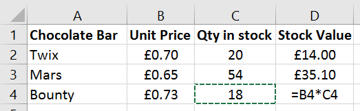
Example: =
However, this formula packs its biggest punch when you use it to include the value of other cells in any mathematical statement. For example, take a look at ‘Example: =’. In cell D4 I’ve typed =B4*C4, once I hit ‘enter’ the answer will be £13.14. This is because the formula in D4 is asking me to multiply £0.73 (the value of B4) by 18 (the value of C4). Using a formula means that if I need to change the values of cells B4 or C4, the value in cell D4 changes automatically. Neat!
=Sum
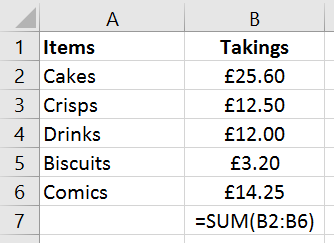
Example: =SUM
This helpful formula can quickly calculate the total value of a ‘range’. In this example (see ‘Example: =SUM’), I’ve listed how much takings I’ve made from each item at a ‘tuck shop’. If I type =SUM(B2:B6) into cell B7, this will add-up all of the values in cells B2, B3, B4, B5 and B6 and put the total in cell B7. (B2:B6) is the range and tells your spreadsheet which values to add-up.
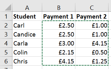
=SUM range
This range can be adapted to calculate values over several columns and rows. In example ‘=SUM range’ I’d like to use =SUM to calculate the total value of all payments received. The formula I would use is =SUM(B2:C6) where B2 represents the top left hand corner and C6 represents the bottom right hand corner of the range of values I’d like to add-up.
=Average
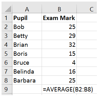
Example: =AVERAGE
Imagine that your class has just taken an exam. You’ve collected in the marks and you want to know the class average. In this example:
- Pupil Names are listed in Column A
- Exam Marks are listed in Column B
- You want the average exam mark to appear in cell B9
To calculate the average type =AVERAGE(B2:B8) into cell B9. Press enter and the calculation will be performed for you. If you change any of the exam marks, the average mark will also change. This formula tells the spreadsheet to find the average mark in cells B2 to B8 – you can change B2:B8 to cover any range.
Top Tip – When you press enter, after you’ve typed your formula, you may find that the result is not a whole number i.e. there are lots of numbers after the decimal point. Use the ‘decrease decimal’ button in your spreadsheet to change this.
=Max
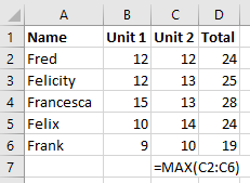
Example: =MAX
Let’s suppose that you have a very long list of exam results and you want to quickly identify the highest mark achieved. The MAX formula is the perfect solution!
In this example, I want to find the highest mark achieved in unit 2. All of the unit 2 marks, for each of the students, are listed in column C. To reveal the highest mark, the formula is =MAX(C2:C6). Remember, C2:C6 is representing the range of the marks that you want your spreadsheet to look at when working out what the highest mark is. After typing this formula, press Enter, and the highest mark will appear. My example is obviously very short and you could probably see the highest mark quicker than even using this formula! This formula, however, is perfect for a very long list where it may not always be obvious what the highest mark is.
Now you can calculate the highest mark, it’s likely that you’ll also want to calculate the lowest…
=Min
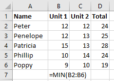
Example: =MIN
Step forward =MIN The spreadsheet formula to calculate the lowest value in a range of values. It’s essentially the opposite of =MAX and in this example, I’d like to quickly see the lowest value in the unit 1 exam. To do this, I type =MIN(B2:B6) into cell B7.
Like any spreadsheet formulas with a range e.g. (B2:B6), you can adapt this part of the formula to fit the requirements of your spreadsheet.
=CountIf
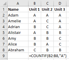
Example: =COUNTIF
Let’s suppose you have a very long table detailing the results of an exam. You’d like to see how many students achieved a particular grade. This is where you’ll need to use =CountIf. This handy formula calculates how many words, letters or numbers meet your search criteria.
For example, in this small table I’d like to calculate, in cell B9, how many students achieved a grade A for unit 1. The formula =COUNTIF(B2:B8,"A") tells the spreadsheet to look at all of the data in cells B2, B3, B4, B5, B6, B7 and B8 and count how many times the letter ‘A’ appears. Once you press ‘enter’, the cell in this example would give the answer as 3.
You can change the search criteria, in this example it is the letter ‘A’, to a number, a word or even a phrase. COUNTIF is a really helpful formula for teachers, particularly when you have large amounts of data and you need to quickly know how often a particular grade or result appears in a table.
=If
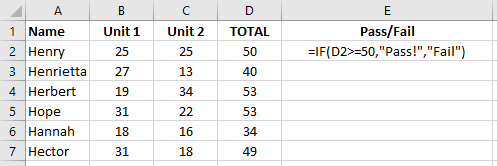
Example: =IF
In this table, Column D details the total of unit 1 and unit 2 using the =SUM formula (see above). I’d like column E to state ‘Pass!’ if a student has scored 50 or more, and ‘Fail’ if the student scored less than 50. The IF formula can help you do this.
Essentially the IF formula is made up of two parts: check whether a statement is true and if it is, do something. If the statement is false then do something else. In cell E2 I’ve typed =IF(D2>=50,"Pass!","Fail"). This means ‘Check the value of cell D2. If it is equal to or greater than 50 then display Pass!. Otherwise, display Fail.’
Spreadsheet Formulas: Put them all together and what do you get?
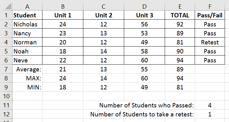
SUM, COUNTIF, AVERAGE, MAX, MIN and IF
In this table:
- =SUM is used in column E to calculate the total values of each unit for each student.
- =IF is used in column F determine whether a student has passed (pass mark is 83) or requires a retest.
- =COUNTIF is used in cells F11 and F12 to show how many students have passed or require a retest.
- =MAX, =MIN and =AVERAGE are used in rows 7, 8 and 9 to show the highest, lowest and average marks in each unit as well as for the total marks in column E.
Spreadsheet formulas are essential knowledge for teachers and this webpage list just a fraction of the available formulas available. If you’ve got any thoughts on formulas or have a spreadsheet story to share why not ‘join the discussion’ below?
Further spreadsheet help:
 Currently the Head of e‑Learning and a teacher of Music and Computing at a large school in